Convex Optimization: Convex set
- Affine and convex sets
- Cones (锥)
- Some important examples
- 1. Hyperplane and halfspace
- 2. Euclidean ball and ellipsoid(Euclidean 球和椭球)
- 3. Norm balls and norm cones
- 4. Polyhedra
- 5. The positive semidefinite cone (半正定锥)
- Remark1: Positive definite matrices and Positive semidefinite matrices
- Remark 2: Various norms
- Remark3: Singular matrix and Nonsingular matrix
- Remark4 :Singular Value Decomposition(SVD)
- Operations that preserve convexity (保凸运算)
- Generalized inequalities
- Separating and supporting hyperplanes( 分离和支持超平面)
- Dual cones and generalized inequalities(对偶锥)
Affine and convex sets
仿射集合和凸集
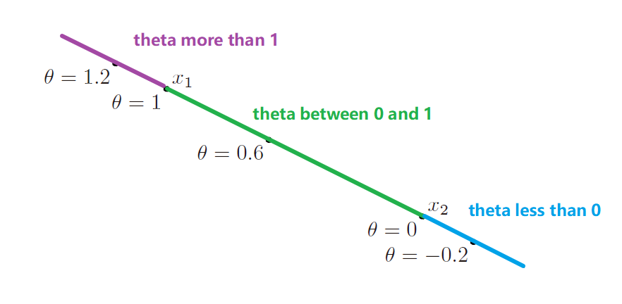
1. Lines and line segments
$y=\theta x_1+(1-\theta)x_2$,$x_1 \ne x_2$。
-
if $\theta \in R$,y就是个line
-
if $0\le \theta \le1$,y就是line segments
2. Affine set (仿射集)
A set $C \in R^n$ is affine if the line through any two distinct points in $C$ lies in $C$, i.e. if for any $x_1, x_2 ∈ C$ and $\theta \in R$, we have $\theta x_1+(1-\theta)x_2 \in C$.
对于集合C中的任意两个不相同的点$x_1,\ x_2$, 点$\theta x_1+(1-\theta)x_2$也在集合C中,且对于$\theta \in R$都成立,则C就叫仿射集。
Affine combination (仿射组合):$\theta_1x_1+…+\theta_kx_k$ (where $\theta_1+…+\theta_k=1$) 就是点$x_1,..,x_k$的仿射组合
| Subspace (子空间): $V=C-x_0={x-x_0 | x \in C }$ (C is a affine set) |
| Affine hull (仿射包) aff $C={\theta_1x_1+…+\theta_kx_k | x_1,..,x_k \in C,\theta_1+…+\theta_k=1}$ |
- The affine hull is the smallest affine set tha contains $C$
- Affine dimension (仿射维度): the affine dimension of a set $C$ is the dimension of its affine hull.
-
relative interior (相对内部): if the affine dimension of a set $C \subseteq R^n$ is less than $n$, then the affine set aff $C \ne R^n$. so the relative interior of the set $C$ is **relint **$C={x \in C B(x,r) \cap \rm{aff} C \subseteq C\rm{\ for\ some\ }r >0 }$, where $B(x,r)={y \left|y-x \right| \le r}$. - relative boubdary (相对边界): cl $C$ is the closure of $C$
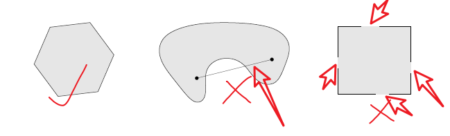
3. Convex sets (凸集)
A set $C$ is convex if the line segment between any two points in $C$ lies in $C$, i.e. if for any $x_1, x_2 ∈ C$ and any $0\le\theta \le1$, we have $\theta x_1+(1-\theta)x_2 \in C$.
对于集合C中的任意两个不相同的点$x_1,\ x_2$, 点$\theta x_1+(1-\theta)x_2$也在集合C中,且对于$0\le\theta \le1$都成立,则C就叫凸集。
Convex combination (凸组合):$\theta_1x_1+…+\theta_kx_k$ (where $\theta_1+…+\theta_k=1$, $\theta_i \ge 0,i=1,…,k$) 就是点$x_1,..,x_k$的凸组合
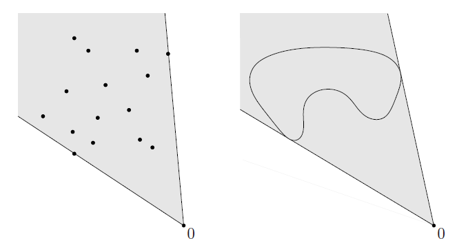
| Convex hull (凸包): conv $C={\theta_1x_1+…+\theta_kx_k | x_1,..,x_k \in C,\theta_1+…+\theta_k=1,\theta_i\ge0,i=1,…,k}$ |
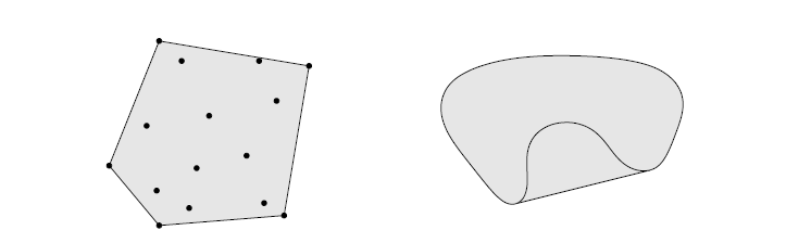
Left. 阴影部分就是那15个点形成的凸包
Right. 阴影部分是Kidney shaped set的凸包
Cones (锥)
Convex cone (凸锥): $\theta_1x_1+\theta_2x_2 \in C$ ,for any $x_1,x_2 \in C$ and $\theta_1,\theta_2\ge0$
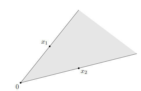
Conic combination (锥组合):$\theta_1x_1+…+\theta_kx_k$ (where $\theta_1+…+\theta_k\ge1$) 就是点$x_1,..,x_k$的锥组合(or nonnegation linear combination)
| Conic hull (锥包):${\theta_1x_1+…+\theta_kx_k | x_1,..,x_k \in C,\theta_i\ge0,i=1,…,k}$ |
下图就是两个集合的锥包
Some important examples
1. Hyperplane and halfspace
| **Hyperplane (超平面): **${x | a^Tx=b}$, where $a\in R^n,a\ne0,b\in R$ |
- $a$: normal vector (法线)
- $b$ determines the offset of the hyperplane from the origin
- hyperplanes are affine and convex
-
${x a^T(x-x_0)=0}$
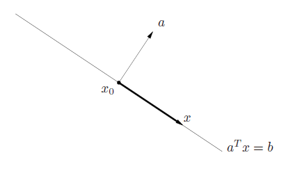
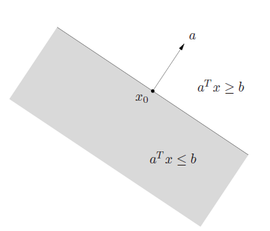
| Halfspace (半平面):${x | a^Tx \le b}$, where $a\ne0$ |
- halfspaces are convex, but not affine.
- $a$ is the outward normal vector.
-
open halfspace: ${x a^Tx < b}$
2. Euclidean ball and ellipsoid(Euclidean 球和椭球)
| **Euclidean ball: **$B(x_c,r)={x | \left| x-x_c \right|_2 \le r}={x | (x-x_c)^T (x-x_c)\le r^2}={x_c+ru | \left| u\right |_2 \le 1}$ |
- $\left | \cdot \right|$ denotes the Euclidean norm
| Ellipsoid: $\cal E={x | (x-x_c)^TP^{-1}(x-x_c)\le1}$ where$P=P^T\succ0$ |
- $P$ is symmtric and positive definite (对称,正定)。
- a ball is an ellipsoid with $P=r^2I$
-
$\cal E={x_c+Au \left | u\right |_2 \le 1}$ where A is square and nonsingular (非奇异的方阵)
3. Norm balls and norm cones
| **Norm ball (范数球): ** ${x | \left|x-x_c \right |\le r}$ |
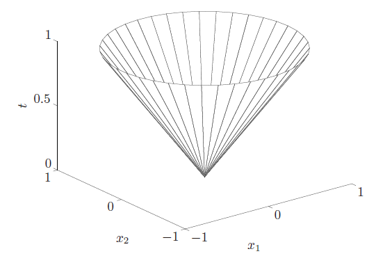
| **Norm cone (范数锥): ** $C={(x,t) | \left|x \right |\le t} \sube R^{n+1}$ |
- norm balls and cones are convex
4. Polyhedra
Polyhedron (多面体): ${\cal P}={a_j^Tx \le b_j,j=1,…,m,c_j^Tx=d_j,j=1,…,p}$
Polyhedra是Polyhedron的复数
-
$Ax \preceq b$, $Cx=d$, where $A \in R^{m \times n}, C \in R^{p \times n}$
-
$\preceq$ is componentwise inequality (分量不等式)
也就是前面矩阵按照每个元素小于等于后面矩阵的对应元素。
-
* Simplexes 单纯形
-
* Convex hull description of polyhedra
Polytope (多胞形):A bounded polyhedron is sometimes called a polytope.
Polyhedron和polytope有的教材会翻过来定义。不用太追究就好。
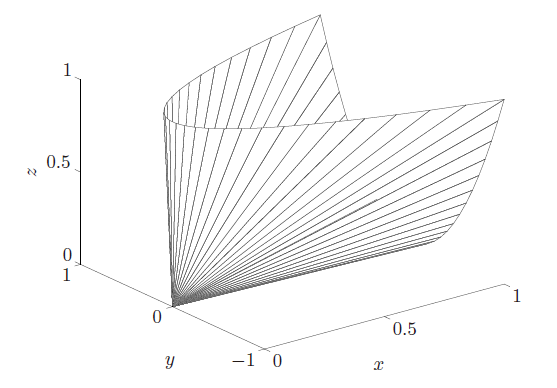
5. The positive semidefinite cone (半正定锥)
-
$S^n$ denotes symmetric $n \times n$ matrix, $S^n={X\in R^{n\times n} X=X^T}$, which is a vector space with dimension $n(n+1)/2$ 这里向量空间维度为什么是$n(n+1)/2$呢?
比如矩阵$X = \left[ {\begin{array}{*{20}{c}}x&y\y&z\end{array}} \right]\in S^n$。因为要保持对称,所以副对角线的元素都是$y$, 因此对于$n=2$的向量空间维度为3。
再如果$X\in S_+^n$是一个半正定对称矩阵的话。
则满足$x\ge 0,z\ge0,xz\ge y^2$。所以可得到一个Positive semidefinite cone.
-
$S_+^n$ denotes the set of symmetric positive semidefinite matrix, $S_+^n={X\in S^n X\succeq0 }$ -
$S_{++}^n$ denotes the set of symmetric positive definite matrix, $S_+^n={X\in S^n X\succ 0 }$
Remark1: Positive definite matrices and Positive semidefinite matrices
参考有人总结的文章浅谈「正定矩阵」和「半正定矩阵」
【定义1】给定一个大小为$n \times n$ 的实对称矩阵$A$,若对于任意长度为$n$的非零向量$x$,有$x^TAx>0$恒成立,则矩阵 $A$是一个正定矩阵。
【定义1】给定一个大小为$n \times n$ 的实对称矩阵$A$,若对于任意长度为$n$的非零向量$x$,有$x^TAx \ge0$恒成立,则矩阵 $A$是一个半正定矩阵。
正定矩阵和半正定矩阵的直观解释
若给定任意一个正定矩阵$A\in \cal R^{n \times n}$和一个非零向量 $x\in \cal R^{n}$ ,则两者相乘得到的向量$y=Ax\in \cal R^n$与向量$x$角恒小于$\frac{\pi}{2}$ . (等价于: $x^TAx>0$)
若给定任意一个正定矩阵$A\in \cal R^{n \times n}$和一个非零向量 $x\in \cal R^{n}$ ,则两者相乘得到的向量$y=Ax\in \cal R^n$与向量$x$角恒小于或等于$\frac{\pi}{2}$ . (等价于: $x^TAx\ge0$)
根据上面的理解,在结合之前在Essence of Linear Algebra系列笔记整理的学习中对线性代数的理解。
将向量$x$作变换矩阵为$A$的线性变换,得到向量新的向量$Ax$, 则$\vec {Ax}$与原来$\vec x$的夹角则决定了变换矩阵$A$是正定的还是半正定的。
正定矩阵的性质
-
正定矩阵的行列式恒为正;
-
实对称矩阵$A$正定当且仅当$A$与单位矩阵合同;
合同变换(congruent transformation)是指在平面到自身的一一变换下,任意线段的长和它的像的长总相等,这种变换也叫做全等变换,或称合同变换。
-
两个正定矩阵的和是正定矩阵;
-
正实数与正定矩阵的乘积是正定矩阵。
正定矩阵的等价命题
- $A$是正定矩阵;
- $A$的一切顺序主子式均为正;
- $A$的一切主子式均为正;
- $A$的特征值均为正;
- 存在实可逆矩阵$C$,使$A=C’C$;
- 存在秩为$n$的$m\times n$实矩阵$B$,使$A=B’B$;
- 存在主对角线元素全为正的实三角矩阵$R$,使$A=R’R$
Remark 2: Various norms
此部分主要参考了0范数,1范数,2范数的区别
向量范数
| 1-范数:$\left | x\right |1=\sum\limits{i = 1}^N {\left | \right | }$ |
2-范数:$\left | x\right |2=\sqrt{\sum\limits{i = 1}^N {x_i^2} }$ ,也叫Euclidean norm/distance
| $\infty$-范数: $\left | x\right |_\infty=\mathop }\limits_i {\left | \right | }$ |
| $-\infty$-范数: $\left | x\right |_{-\infty}=\mathop }\limits_i {\left | \right | }$ |
| p-范数:$\left | x\right |p=\left(\sum\limits{i = 1}^N {\left | x_i \right | ^p}\right)^{\frac{1}{p}} $ |
矩阵范数
| 1-范数:$\left | A\right |1=\mathop }\limits_j \sum\limits{i = 1}^m {\left | } \right | }$, 列和范数 |
2-范数:$\left | A\right |_2=\sqrt{\lambda_1}$ ,$\lambda_1$ 为$A^TA$的最大特征值,谱范数
| $\infty$-范数:$\left | A\right |\infty=\mathop }\limits_i \sum\limits{j = 1}^n {\left | } \right | }$ , 行和范数 |
| F-范数:$\left | A\right |F=\left(\sum\limits{i = 1}^m \sum\limits_{j = 1}^n {\left | a_{i,j}\right | ^2}\right)^{\frac{1}{p}} $, Frobenius范数 |
核范数:$\left | A\right |*= \sum\limits{i = 1}^n { \lambda_i }$, $\lambda_i$是矩阵$A$的奇异值
一下是不同的norm对应的曲线。
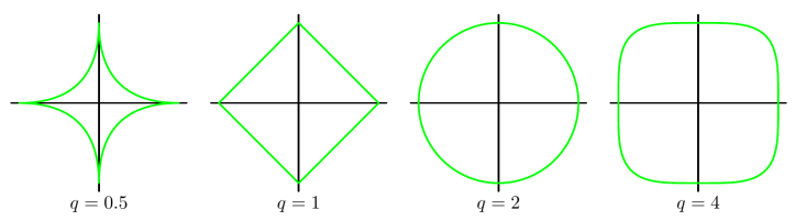
上图中,可以明显看到一个趋势,即$q$越小,曲线越贴近坐标轴,$q$越大,曲线越远离坐标轴,并且棱角越明显。那么 $q=0 $和 $q=\infty$ 时极限情况如何呢?猜猜看。
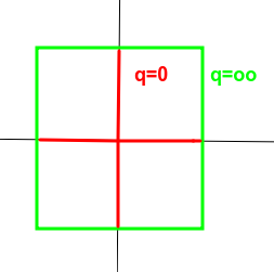
答案就是十字架和正方形。除了图形上的直观形象,在数学公式的推导中,$q=0 $和 $q=\infty$时两种极限的行为可以简记为非零元的个数和最大项。即0范数对应向量或矩阵中非零元的个数,无穷范数对应向量或矩阵中最大的元素。
Remark3: Singular matrix and Nonsingular matrix
Singular matrix (奇异矩阵): 行列式为0的矩阵
Nonsingular matrix (非奇异矩阵): 行列式不为0 的矩阵
- 一个矩阵非奇异当且仅当它的行列式不为零。
- 一个矩阵非奇异当且仅当它代表的线性变换是个自同构。
- 一个矩阵半正定当且仅当它的每个特征值大于或等于零。
- 一个矩阵正定当且仅当它的每个特征值都大于零。
- 一个矩阵非奇异当且仅当它的秩为n
Remark4 :Singular Value Decomposition(SVD)
奇异值分解这部分主要参考了奇异值分解(SVD)
1. 回顾特征值和特征向量
$Ax=\lambda x$
where $A\in R^{n\times n}, x\in R^n$. hence, $\lambda$ is its eigenvalue, $x$ is the eigenvector of $\lambda$.
求出特征值和特征向量有什么好处呢? 就是我们可以将矩阵A特征分解。如果我们求出了矩阵$A$的$n$个特征值$\lambda_1 \le \lambda_2 \le …\le\lambda_n$,以及这$n$个特征值所对应的特征向量$w_1,w_2,…,w_n$.
那么矩阵A就可以用下式的特征分解表示:
$A=W\Sigma W^{-1}$
其中$W$是这$n$个特征向量所张成的$n \times n$维矩阵, 而$\Sigma $为这$n$个特征值为主对角线的$n \times n$维矩阵。
一般我们会把W的这n个特征向量标准化,即满足$\left | w_i\right |_2=1$ ,或者$ w_i^T w_i=1$ ,此时W的
$n$个特征向量为标准正交基,满足$W^TW=I$, 即$W^T=W^{-1}$,也就是说$W$为酉矩阵。
这样我们的特征分解表达式可以写成
$A=W \Sigma W^{T}$
注意到要进行特征分解,矩阵A必须为方阵。
那么如果A不是方阵,即行和列不相同时,我们还可以对矩阵进行分解吗?答案是可以,此时我们的SVD登场了。
2. SVD的定义
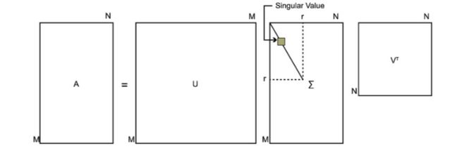
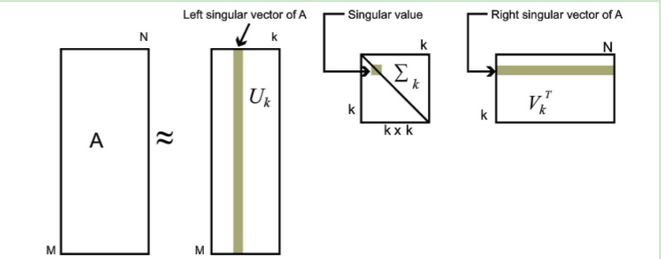
SVD也是对矩阵进行分解,但是和特征分解不同,SVD并不要求要分解的矩阵为方阵。假设我们的矩阵$A$是一个$m \times n$的矩阵,那么我们定义矩阵$A$的SVD为:
$A=U \Sigma V^T$
其中$U$是一个$m \times m$的矩阵, $\Sigma$ 是一个$m \times n$的矩阵,除了主对角线上的元素以外全为0,主对角线上的每个元素都称为奇异值, $V$是一个$n \times n$ 的矩阵。$U$ 和$V$都是酉矩阵,即满足$U^TU=I, V^TV=I$ 。下图可以很形象的看出上面SVD的定义:
那么我们如何求出SVD分解后的$U,\Sigma,V$这三个矩阵呢?
如果我们将$A$的转置和$A$做矩阵乘法,那么会得到$n\times n$的一个方阵$A^TA$。既然$A^TA$是方阵,那么我们就可以进行特征分解,得到的特征值和特征向量满足下式:
$(A^TA)v_i=\lambda_iv_i$
这样我们就可以得到矩阵 $A^TA$ 的$n$个特征值和对应的$n$个特征向量$v$了。将 $A^TA$ 的所有特征向量张成一个$n \times n$的矩阵$V$,就是我们SVD公式里面的$V$矩阵了。一般我们将$V$中的每个特征向量叫做$A$的右奇异向量。
如果我们将A和A的转置做矩阵乘法,那么会得到$m\times m$的一个方阵 $AA^T$ 。既然 $AA^T$ 是方阵,那么我们就可以进行特征分解,得到的特征值和特征向量满足下式:
$(AA^T)u_i=\lambda_iu_i$
这样我们就可以得到矩阵 $AA^T$ 的$m$个特征值和对应的$m$个特征向量$u$了。将 $AA^T$ 的所有特征向量张成一个$m \times m$的矩阵$U$,就是我们SVD公式里面的$U$矩阵了。一般我们将$U$中的每个特征向量叫做$A$的左奇异向量。
$U$和$V$我们都求出来了,现在就剩下奇异值矩阵$\Sigma$没有求出了.由于$\Sigma$除了对角线上是奇异值其他位置都是0,那我们只需要求出每个奇异值$\sigma$就可以了。我们注意到:
$A=U \Sigma V^T \Rightarrow AV=U \Sigma V^TV \Rightarrow AV=U\Sigma \Rightarrow Av_i=\sigma_iu_i \Rightarrow \sigma_i=\frac{Av_i}{u_i}$
这样我们可以求出我们的每个奇异值,进而求出奇异值矩阵$\Sigma$。
$A=U \Sigma V^T \Rightarrow A^T=V \Sigma U^T \Rightarrow A^TA=V\Sigma U^TU \Sigma V^T=V\Sigma^2V^T$
以看出我们的特征值矩阵等于奇异值矩阵的平方,也就是说特征值和奇异值满足如下关系:
$\sigma_i=\sqrt{\lambda_i}$
3. SVD的一些性质
对于奇异值,它跟我们特征分解中的特征值类似,在奇异值矩阵中也是按照从大到小排列,而且奇异值的减少特别的快,在很多情况下,前10%甚至1%的奇异值的和就占了全部的奇异值之和的99%以上的比例。
也就是说,我们也可以用最大的$k$个的奇异值和对应的左右奇异向量来近似描述矩阵。
也就是说:
$A_{m\times n}=U_{m\times m}\Sigma_{m\times n}V_{n\times n}^T \approx U_{m\times k}\Sigma_{k\times k}V_{k\times n}^T$
其中$k$要比$n$小很多,也就是一个大的矩阵A可以用三个小的矩阵$U_{m\times k},\Sigma_{k\times k},V_{k\times n}^T$来表示。如下图所示,现在我们的矩阵$A$只需要灰色的部分的三个小矩阵就可以近似描述了。
由于这个重要的性质,SVD可以用于PCA降维,来做数据压缩和去噪。也可以用于推荐算法,将用户和喜好对应的矩阵做特征分解,进而得到隐含的用户需求来做推荐。同时也可以用于NLP中的算法,比如潜在语义索引(LSI)。
下面我们就对SVD用于PCA降维做一个介绍。
4. SVD用于PCA
PCA降维,需要找到样本协方差矩阵$X^TX$的最大的$d$个特征向量,然后用这最大的$d$个特征向量张成的矩阵来做低维投影降维。可以看出,在这个过程中需要先求出协方差矩阵$X^TX$,当样本数多样本特征数也多的时候,这个计算量是很大的。
注意到我们的SVD也可以得到协方差矩阵$X^TX$最大的$d$个特征向量张成的矩阵,但是SVD有个好处,有一些SVD的实现算法可以不求先求出协方差矩阵$X^TX$,也能求出我们的右奇异矩阵$V$。也就是说,我们的PCA算法可以不用做特征分解,而是做SVD来完成。这个方法在样本量很大的时候很有效。实际上,scikit-learn的PCA算法的背后真正的实现就是用的SVD,而不是我们我们认为的暴力特征分解。
另一方面,注意到PCA仅仅使用了我们SVD的右奇异矩阵,没有使用左奇异矩阵,那么左奇异矩阵有什么用呢?
假设我们的样本是$m \times n$的矩阵$X$,如果我们通过SVD找到了矩阵$XX^T$最大的$d$个特征向量张成的$m\times d$维矩阵$U$,则我们如果进行如下处理:
$X_{d \times n}^\prime =U_{d\times m}^TX_{m \times n}$
可以得到一个$d\times n$的矩阵$X^\prime$,这个矩阵和我们原来的$m\times n$维样本矩阵$X$相比,行数从$m$减到了$d$,可见对行数进行了压缩。
左奇异矩阵可以用于行数的压缩。
右奇异矩阵可以用于列数即特征维度的压缩,也就是我们的PCA降维。
SVD作为一个很基本的算法,在很多机器学习算法中都有它的身影,特别是在现在的大数据时代,由于SVD可以实现并行化,因此更是大展身手。
SVD的缺点是分解出的矩阵解释性往往不强,有点黑盒子的味道,不过这不影响它的使用。
Operations that preserve convexity (保凸运算)
1. Intersection (交集)
the intersection of (any nomber of) convex sets is convex
example:
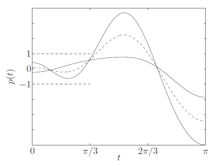
$S={ x\in R^m \left p(t)\right \le1 for t \le\pi/3 }=\cap_{ t \le\pi/3}{ x p(t) \le 1}$ 其中$p(t)=x_1cost+x_2cos2t+\cdot\cdot\cdot +x_mcosmx$
- 证明S(t)是凸的
图中两个实线是随机选取的在$ t \le\pi/3$时满足$ p(t) \le 1$的曲线。相当于在集合中选取的两个点$(x,y)$,然后看$\theta x+(1-\theta)y$是否也满足$ p(t) \le 1$,即也在集集合中。图中的虚线就是取的$\theta=1/2$时的情况,可以看到在$ t \le\pi/3$仍然满足$ p(t) \le 1$,即$\theta x+(1-\theta)y$也在集集合中。得证$S$是凸集
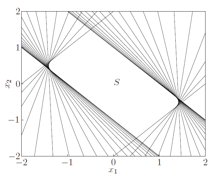
- 下图绘制出了当$m=2$时的集合图
$S={ x\in R^m \left x_1cost+x_2cos2t \right \le1 for t \le\pi/3 }$
其中$x_1cost+x_2cos2t$是一个line,$\left x_1cost+x_2cos2t \right \le1$就是两个line和中间的部分组成的slab(平板)。当$t$取值不同时,曲线的斜率也不同。就构成了无数个slabs。将这些slabs取交集便是$S$
2. Affine function
$f:R^n \to R^m$
$f(x)=Ax+b$, where $A \in R^{m \times n}, b\in R^m$
| image: $f(S)={ f(x) | x \in S}$ |
| **inverse image: ** $f^{-1}(S)={ x | f(x) \in S}$ |
Both image and inverse image can peserve convexity
这里f(x)也可以说是linear,但是linear是informal说法,affine比较正式
Examples
-
scalling: $\alpha S={\alpha x x\in S}$ -
**translation: **$S+a={x+a x\in S}$ -
**projection: ** $T={ x\in R^m (x_1,x_2)\in S\sube R^m\times R^n \rm{for\ some\ } x_2\in R^n}$ -
**sum: **$S_1+S_2={x+y x\in S_1,y\in S_2}$ -
**Cartesian product: **$S_1\times S_2={(x_1,x_2) x_1\in S_1,x_2\in S_2}$ -
**partial sum: ** $S={(x,y_1+y_2) (x,y_1)\in S_1,(x,y_2)\in S_2}$ -
**polyhedron: **${x Ax \preceq b,Cx=d }={ x f(x)\in R_+^m\times{ 0} }$, $f(x)=(b-Ax,d-Cx)$ -
**solution of linear matrix inequlity: ** ${x A(x) \preceq B}={ x f(x)\in R_+^m}$, $f(x)=B-A(x),f:R^n \to R^m$ -
Hyperbolic cone (双曲线锥):${x x^TPx\le(c^Tx)^2, c^T x \ge 0 }=f^{-1}({ (z,t) z^Tz\le t^2,t \ge 0 })$, where $P\in S_+^n,c\in R^n,f(x)=(P^{1/2}x,c^Tx)$.
3. Linear-fractional and perspective function
perspective function: **$P:R^{n+1} \to R^n$ with domain **dom $P=R^n \times R_{++}$, $P(z,t)=z/t$
-
perspective function(透视函数) 也是保凸的
-
the inversr image is also convex $P^{-1}(C)={(x,t)\in R^{n+1} x/t\in C,t>0}$ -
可将之形象的理解成小孔成像,将3D图像映射到2D底板上。
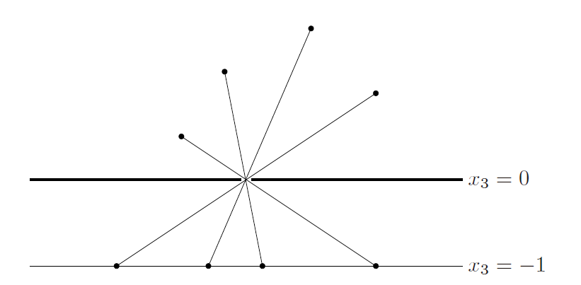
$x_3$相当于第$n+1$列的数值都变成了全部相同的数字,因此直接舍去。
Linear-fractional function
$g:R^n \to R^{m+1}$, $g(x)=\left[ \begin{array}{l}{\rm{A}}\{c^T}\end{array} \right]x + \left[ \begin{array}{l}b\d\end{array} \right]$. where $A\in R^{m \times n},b\in R^m,c \in R^n$
| $f:R^n \to R^m, $$f=P \circ g$, $f(x)=\frac{Ax+b}{c^Tx+d}, \mathbf{dom}f={ x | c^Tx+d >0}$ |
Generalized inequalities
1. proper cone(正常锥)
- $K$ is convex
- $K$ is closed
- $K$ is solid, which means it has nonempty interior.(实心的)
- $K$ is pointed, which means that it contains no line(尖的)
so, $K \sube R^n$ is called a proper cone
2. partical ordering(偏序)
- partical ordering:$x \preceq_K y \Leftrightarrow y-x \in K$
- strict partical ordering:$x \prec_K y \Leftrightarrow y-x \in {\mathbf{int}}K$
- componentwise inequality
- matrix inequality:
- $S_+^n$ is a proper cone in $S^n$ : positive semidefinite cone
- $X \preceq_K Y \Leftrightarrow Y-X$ is a positive semidefinite
- $X \prec_K Y \Leftrightarrow Y-X$ is a positive definite
3. properties of generalized inequlities
A generalized inequality $\preceq_K$ satisfies many properties
- $\preceq_K$ is preserved under addition(加法保序)
- $\preceq_K$ is transitive (传递性)
- $\preceq_K$ is preserved under nonnegative scaling (非负数乘保序)
- $\preceq_K$ is reflexive: $x\preceq_K x$ (自反性)
- $\preceq_K$ is antisymmetric: if $x\preceq_K y$ and $y\preceq_K x$, then $x=y$(反对称性)
- $\preceq_K$ is preserved under limits(极限运算保序)
A strict generalized inequality $\prec_K$ satisfies
- if $x\prec_K y$ then $x\preceq_K y$
- if $x\prec_K y$ and $u\prec_K v$ then $x+u\prec_K y+v$
- if $x\prec_K y$ and $\alpha > 0$ then $\alpha x\prec_K \alpha y$
- $x\nprec_K y$
- if $x\prec_K y$ , then for $u$ and $v$ small enough,$x+u\prec_K y+v$ .
4. minimum and minimal elements(最小和极小元)
- $x \in S$ is the minimum element of $S$ with respect to $\preceq_K$ if $y\in S \Rightarrow x \preceq_K y$
- $x \in S$ is the minimal element of $S$ with respect to $\preceq_K$ if $y\in S , y\preceq_K x\Rightarrow y=x$
可以对照最小值与极小值的概念理解
Separating and supporting hyperplanes( 分离和支持超平面)
1. Separating hyperplane theorem
| Suppose $C$ and $D$ are nonempty disjoint convex sets, i.e., $C \cap D = \emptyset$. Then there exist $a \ne 0$ and $b$ such that $a^T x \le b$f or all $x \in C$ and $a^T x \ge b$ for all $x \in D$. In other words, the affine function $a^T x−b$ is nonpositive on $C$ and nonnegative on $D$. The hyperplane ${x | a^T x = b}$ is called a separating hyperplane for the sets $C$ and $D$, or is said to separate the sets $C $and $D$. |
- proof of separating hyperplane theorem
- strict separation
2. supporting hyperplane theorem
Suppose $C\sube R^n$, and $x_0$ is a point in its boundary $\mathbf{bd} C$, i.e., $x_0 \in \mathbf{bd}C = \mathbf{cl}C \backslash \mathbf{int}C$. If $a \ne 0$ satisfies $a^T x ≤ a^T x_0$ for all $x\in C$, then the hyperplane${ x | a^T x = a^T x_0}$ is called a supporting hyperplane to $C$ at the point $x_0$.
Dual cones and generalized inequalities(对偶锥)
1. Dual cones
| $K^* = {y | x^T y ≥ 0 {\rm{\ \ for\ all\ }} x \in K}$ is called the dual cone of K, which is a cone. |
2.Dual generalized inequalities
- $x \preceq K y$ if and only if $\lambda ^T x \le \lambda^T y$ for all $λ \ \succeq{K^*} 0$.
- $x \prec K y$ if and only if $\lambda ^T x < \lambda^T y$ for all $λ \ \succeq{K^*} 0$, $\lambda \ne0$.
课后习题我也做了EE364a的作业,emmm….自己做真的是什么都不会,不知道怎么下手,我是看了看答案理解了再自己写一遍。贴上来没啥意思。就不贴习题了。
对本文有任何问题,请在下面评论: